Read OEE and Production Counts

OEE is one number, but three different problems can pull it down. This lesson shows you how to read OEE, work out which part is the problem, and check the production counts behind it.

How OEE Is Made​

OEE is Availability × Performance × Quality. Each part answers a different question.

PartHow it's worked outA low number means
AvailabilityRuntime / (runtime + unplanned downtime). Planned downtime, such as a clean in place, is left out.The machine stopped too much.
PerformanceInfeed count / (infeed rate × runtime)The machine ran slower than its standard rate.
Quality(Infeed count - waste count) / infeed countToo much of what went in was scrapped.

Performance uses infeed and runtime, so downtime and scrap don't distort it. Quality needs at least two counts. With only one, quality shows 100%.

Reference Materials: OEE Calculation - Availability, performance and quality.

OEE Calculation​

OEE is a widely accepted lean manufacturing standard, and extensive resources are available online. Here, we�ll focus primarily on how it is calculated and how it can be customized.

The term OEE was invented in the 1960s by the creator of the Total Productive Maintenance system, Seiichi Nakajima. OEE is expressed as a percentage from 0 to 100, where an OEE score of 100 percent would indicate that a manufacturing line or cell was producing only good parts at the anticipated production rate with no unexpected stops.

OEE is calculated by multiplying Availability * Performance * Quality


Read the OEE Chart​

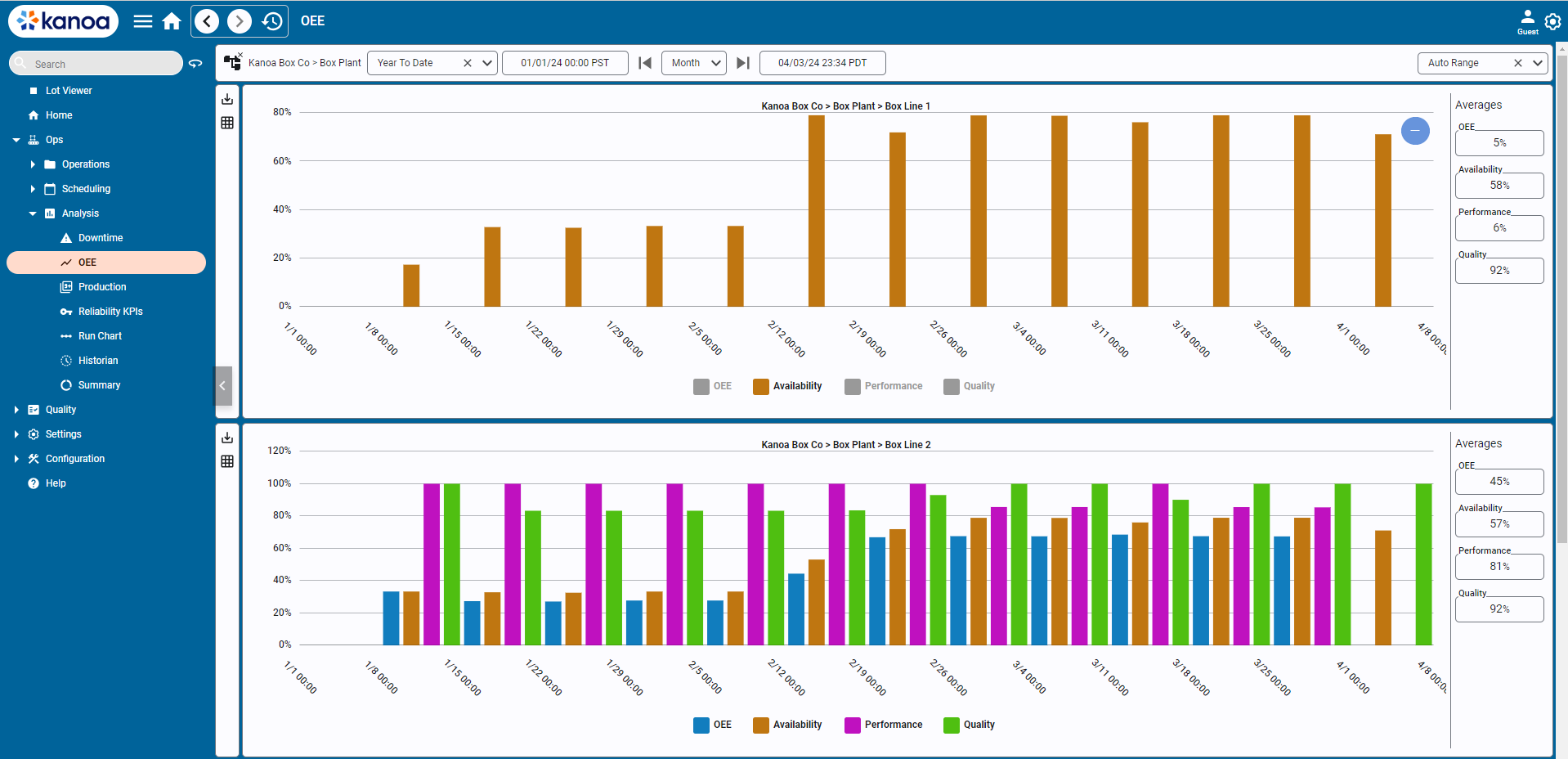
OEE report

The OEE chart shows the parts of OEE side by side over time.

  1. Open Ops → Analysis → OEE.
  2. Choose an asset, or an area or site to include everything under it.
  3. Choose a date range.
  4. Read the chart. Kanoa picks the interval for you: hourly for one day, daily for several days, weekly across months. You can choose another, but a year by hour doesn't render well.
  5. Read the average OEE, availability, performance and quality on the right.
  6. Click a name in the chart legend to hide or show that plot.

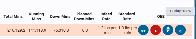
OEE is colour-coded wherever it's shown: green is good, orange is a warning and red is bad. The thresholds are set per asset.
OEE colour coding

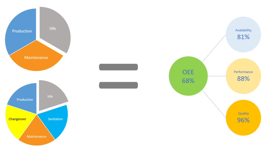
Modes as pies

tip

The same OEE can hide very different utilization, as in these mode pies. Look at where the asset's time went, not only the percentage.

Find Which Part Drove It​

Compare the three averages. The lowest part is where to look next.

  • Low availability: go to the downtime reasons in the previous lesson.
  • Low performance: look at speed-loss events and their reasons.
  • Low quality: look at the scrap reasons, below.

Loss Analysis does this in minutes. It shows OEE with its parts at the top, then the three loss cards, with the biggest marked. See the previous lesson.

Reference Materials: Loss Analysis figures - TEEP, utilization, OEE and its parts.

The figures at the top​

FigureWhat it is
TEEPValuable time / calendar time: what the assets made of every hour in the range
UtilizationProduction time / calendar time: how much of the range the assets were producing
OEEAvailability x Performance x Quality = valuable time / planned run time
AvailabilityActual run time / planned run time
Performance(Actual run time - performance loss) / actual run time
QualityValuable time / (actual run time - performance loss)

Below them, the time figures show how the time breaks down. They are summed over every asset included, so a one-day range across several assets can add up to days.

  1. Production run time: the time the production runs took. Losses are only counted inside it.
  2. minus Planned downtime (stops with a Planned Downtime state, such as breaks) = Planned run time.
  3. minus the availability loss: unplanned downtime, every stop that is not running or planned and lasts at least Short stop.
  4. minus the performance loss: minor stops, plus speed loss = (standard count - actual count) x cycle time.
  5. minus the quality loss: waste x cycle time.
  6. What is left is Valuable time: good parts made at the standard rate.

Check Production Counts Against Target​

The Production Counts chart shows how an asset's infeed, outfeed and waste built up against its target. The same chart is on the Asset Operation page as the Asset Run Analysis dashboard.
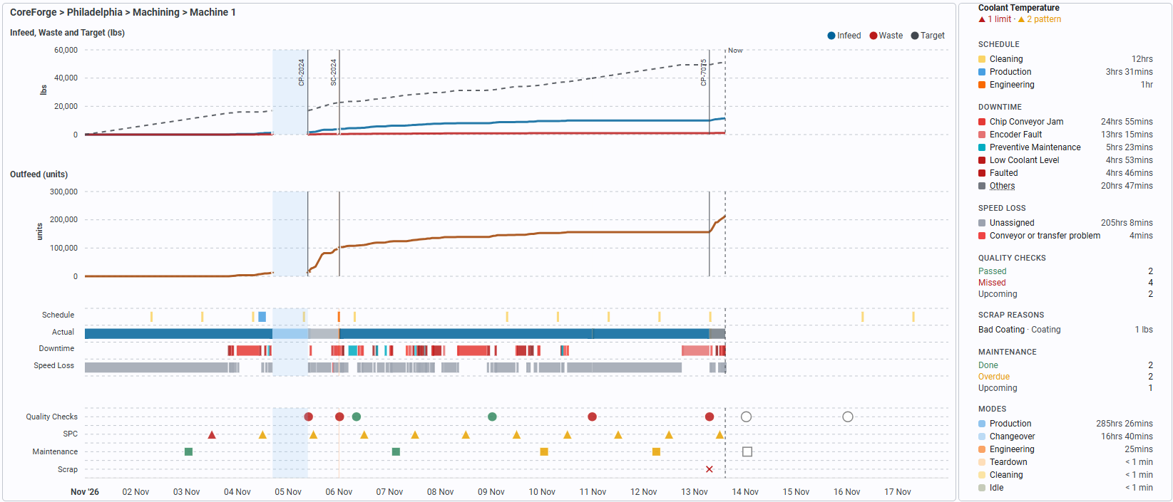
Production Counts chart

  1. Select an OEE asset and a date range, then click Go. The chart covers up to 7 days.
  2. Read the lines. Each is a running total, so it rises while the asset produces and stays flat while it doesn't.
  3. Compare Outfeed with the dashed Target line. The gap shows how far ahead or behind you are.
  4. Look at the Waste line, and at the Scrap row under the timeline.
  5. Hover over the chart to see the totals at that time and what the asset was doing.

Under the counts, the timeline shows what was Scheduled against what Actually ran, with the Downtime and Speed Loss rows. The shading shows time in modes other than Production.

Reference Materials: Reading the Chart - Lines, target, modes and the timeline.

Reading the chart​

Each line is a running total, so it rises as the asset produces and stays flat while it doesn't:

  • Infeed, Outfeed and Waste are the counts recorded while the asset was in a Production mode. Counts made in any other mode (Changeover, Idle, Maintenance and so on) aren't included, and the lines break while the asset isn't in Production.
  • Target (dashed) is the standard rate of the item running, times the production time. Its slope changes when an item with a different standard rate starts, so the gap between Outfeed and Target shows how far ahead of or behind target the asset is at any point in the range.

The lines follow the counts hour by hour, whatever interval the table uses. A count with nothing recorded in the range isn't drawn, and its total is left out of the panel.

Hovering over the chart shows every line's total at that time, with its units, and what the asset was doing under the mouse: the mode with when it started, when it ended and how long it lasted, or for Production, the item, the work order and its required quantity.

When the counts are in different units (for example, infeed and waste in lbs and outfeed in units), the chart is split into two plots stacked on the same time axis, each titled with what it shows. When all the counts are in the same units, there's a single plot.

The chart runs to the end of the date range. When the range ends after now (for example, This Week), the lines stop at a dashed Now line, and the space after it shows the quality checks and maintenance scheduled for the rest of the range.

Zooming in​

Drag across the chart to look at that time more closely: the date selector switches to Custom with the dragged range, and the chart, timeline, events and totals reload for it. A Zoom out icon appears beside the period arrows; each click goes back one step, to the range before the last drag. Picking a range in the date selector clears the zoom steps.

Modes​

The time the asset spent in a mode other than Production is shaded on the chart in that mode's colour. Production isn't shaded; the Actual row of the timeline shows each Production run in its item's colour.

Items​

A vertical line marks each point where the item changed, labelled with the item that started (some labels are left off when changes are close together).

Tooling​

On an asset that uses tooling, a coloured diamond along the top of the chart marks each point where a different tool (a mold, die and so on) was mounted. Each tool keeps one colour, matching the Tooling list in the totals panel. Hover over a diamond to see the tool, when it was mounted and how long it stayed on. Taking a tool off and putting it back on isn't marked as a change, and a tool mounted inside another tool (an insert in a mold base) isn't shown separately.

SPC alerts​

When the asset has measures with SPC checking turned on, a triangle on the SPC row under the timeline marks each interval with an SPC alert: red when a measure went beyond a control or specification limit, amber for a pattern (a run or trend that shows a shift or drift), and grey for too little variation. Hover over a triangle to see the measures and the rules they broke.

The alerts are worked out for the date range with each measure's current limits, using the same rules as the measure's live SPC check. Past alerts aren't stored, so if a measure's limits changed during the range, its earlier values are judged against the new ones.

Timeline​

Under the counts, a timeline shows on the same time axis, row by row:

  • Schedule: the operations scheduled for the asset, in each one's mode colour.
  • Actual: what the asset actually did, a bar for each run in every mode. Production runs are in the item's colour, other modes in the mode's colour, so the Schedule and Actual rows can be compared directly.
  • Downtime: each downtime event, in its state's colour.
  • Speed Loss: each period the asset ran slower than its standard rate (a performance event), in its reason's colour. Automatic speed-loss events show as Unassigned until an operator gives them a reason.

A row with nothing in the range is left out, and the timeline is only as tall as the rows it shows. Very short events are drawn a little wider so they can be seen. Hover over a bar to see its details: the item, work order and required quantity of a run, the state and note of a downtime, or the reason, times and minutes lost of a speed loss.

Quality checks, SPC, maintenance and scrap​

Below the timeline, the asset's quality checks, SPC alerts, maintenance work orders and scrap are marked on the same time axis:

  • Quality Checks (circles): the check sheets scheduled in the range, at the time each was taken (or due, if it wasn't).
  • SPC (triangles): the SPC alerts described above.
  • Maintenance (squares): the maintenance work orders due in the range, on the asset or on a tool mounted on it.
  • Scrap (red crosses and amber diamonds): the waste recorded with a reason (coded scrap), and the hours with a lot of waste recorded without one (uncoded scrap). See Scrap markers below.

Quality and maintenance marks are coloured by status: green for a check passed or a work order done, red for a check failed or missed, amber for overdue, blue for a work order in progress, and an empty grey mark for one still to come. Hover over a mark to see the check sheet or the work order. As on the timeline, a row with nothing in the range is left out, and the plot is left out when the asset has none of these in the range.

Scrap markers​

The Scrap row shows two kinds of marker:

MarkerMeaning
Red cross (✕)Coded scrap: waste counted with a reason (an item state), at the time it was counted.
Hollow amber diamond (◇)Uncoded scrap: an hour in which the waste counted without a reason reached the threshold (5% of the hour's infeed by default).

Coded scrap. Each waste count with a reason gets a cross at the time it was counted. Hover over it to see the reason, its category, the quantity, the item, the work order and the time. Counts that are close together (within 1% of the chart's date range, about a marker's width) are merged into one cross, so several reasons recorded at the same time don't hide each other. The hover of a merged cross lists each reason with its category and quantity, most first, under the number of reasons and their total, for example 3 scrap reasons, 150 units, and the time (or times) they were counted.

Uncoded scrap. Waste that's counted without a reason is on the Waste line but has no count of its own to mark, so the chart works it out by hour:

  1. It takes the hour's waste (the same counts the Waste line uses) and subtracts the coded scrap counted in that hour. What's left is the hour's uncoded waste.
  2. It compares the uncoded waste with the hour's infeed. When it's at least the threshold percentage (5% by default), the hour gets a diamond at its start.

Hover over a diamond to see the uncoded waste, its percentage of the infeed with the threshold it was checked against, and the hour, for example Uncoded waste: 2,000 units, 10% of infeed (marked from 5%), Nov 10, 22:00 to 23:00. Diamonds that are close together are merged in the same way as crosses: the hover gives the number of hours and their total (Uncoded waste in 2 hours, 55.4 lbs), then each hour on its own line.

Some details of how the diamonds are decided:

  • Units. The waste is compared with the infeed when both are counted in the same units. When the waste is in the outfeed's units instead (for example, infeed in lbs, outfeed and waste in units), it's compared with the outfeed. When neither matches, a percentage can't be worked out, so every hour with any uncoded waste gets a diamond, and its hover says what units the waste, infeed and outfeed are in.
  • No infeed. An hour with uncoded waste but no infeed (or outfeed) counted is marked, and its hover says so.

When a cross and a diamond touch, the hover of each also shows the other's text, so whichever one is under the pointer shows both.

The times in the scrap hovers are in your device's time zone, the same as the chart's time axis.

Read the Totals​

The panel on the right of the chart shows totals for the range. It lists each run, and the time in each downtime state and speed-loss reason, longest first. Scrap Reasons lists the waste recorded against each reason, and Uncoded (no reason) is waste with none.

Most sections open something when you click them. Click a run to open its count editor. Click Scrap Reasons to open the Scrap editor.

Code Uncoded Scrap​

Waste with no reason hides what to fix. The Scrap row marks two kinds of waste:

MarkerMeaning
Red cross (✕)Coded scrap: waste counted with a reason.
Hollow amber diamond (◇)Uncoded scrap: an hour where waste with no reason reached 5% of the infeed, by default.

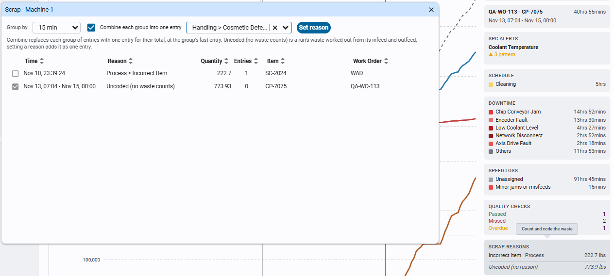
The Scrap editor

  1. In the totals panel, click Scrap Reasons to open the Scrap editor.
  2. Select the rows to code. Select uncoded selects them all.
  3. Pick a reason in the list, then click Set reason.

Clear reason puts selected counts back to uncoded, and Delete removes a wrong count. Delete asks you to click again to confirm.

Reference Materials: Coding Scrap - Group, set, clear and delete waste counts.

Coding scrap​

Clicking Scrap Reasons opens the Scrap editor for the chart's asset and date range, to give waste a reason (code it), change or clear its reason, or delete a waste count that was wrong. It lists:

  • The waste counts, grouped by Group by: 15 min (the default), Entry (each count on its own), Hour or Run. A group holds the counts with the same reason, item, work order and counter, so a group never spans two runs. Each row shows the group's time, its reason (or Uncoded), its quantity and how many counts it holds.
  • Uncoded (calculated): a row for each run whose waste has no waste counts at all. Such a run's waste is calculated from its infeed and outfeed (infeed less outfeed times the package count), so there's no count to code until it's given a reason. It's one row for the whole run, while the chart's Scrap row marks the uncoded waste hour by hour; the editor says so when it shows one.

The Scrap editor

Click rows to select them, then:

  • Set reason: gives the selected rows the reason picked in the list beside it. With Combine each group into one entry ticked (the default), each group's counts are replaced by one count for their total, at the time of the group's last count, with the same item and work order, which keeps the chart's lines where they were and leaves fewer counts to code next time. Unticked, each count keeps its own time and only its reason changes. An Uncoded (calculated) row is added as one count for the run's full waste, a second before the run's end, so the run's waste stays the same.
  • Clear reason (shown once a waste count is selected): sets the selected counts back to uncoded, combined in the same way.
  • Select uncoded (shown when there are two or more uncoded rows): selects them all, to code them with one reason.
  • Delete (shown once a waste count is selected): removes the selected counts. The first click turns it into Confirm Delete; the second deletes. A run left with no waste counts has its waste worked out from its infeed and outfeed again.

With Group by set to Entry, a count's quantity can be changed in the table; it keeps its time. The chart, its totals and the runs refresh after each change.

Not logged in, the editor only shows the waste: it has no controls, checkboxes or buttons. A waste count can also be added from a run's count editor (click the run in the totals panel).

Check Your Understanding​

  1. An asset's OEE is 55%. Availability is 95% and quality is 98%. Which part is the problem?
  2. On the Production Counts chart, how do you see whether the asset is ahead of or behind target?
  3. What does a hollow amber diamond on the Scrap row mean?
Answers
  1. Performance. The machine ran, and little was scrapped, but it ran slower than its standard rate.
  2. Compare the Outfeed line with the dashed Target line. The gap is how far ahead or behind it is.
  3. An hour in which waste counted with no reason reached the threshold, 5% of the infeed by default. The waste needs a reason.